My Two Cents - "Partial Equilibrium Analysis - Part I"

08/30/2010

One of the many tools available to economists and analysts in determining the suitability of fiscal or economic policy is partial equilibrium (PE) analysis. However, many scoff at the notion of using partial equilibrium simply because many of its assumptions are deemed to be too unrealistic. However, for taking a look at the potential benefits (or costs) of a policy such as a tax on a single good, PE is a very valid construct. One of the biggest hot button topics these days in nearly every state is how to raise revenue (rather than cutting costs). One of the traditional cash cows for states is in the form of gasoline taxes. The same goes for the Federal government in this regard. However, as we all know, simply arbitrarily and capriciously taxing a product is not necessarily efficient. In fact it usually isn’t.

Proponents of supplemental gasoline taxes have pointed out that the additional revenue gives the taxing authority resources, which it can use to benefit citizens, increase spending, and generate economic activity. This argument is centered on the belief that government can most efficiently allocate economic resources. Opponents claim that the taxes create an unnecessary and unfair drag on those economic agents (people) who tend to create the most in the way of economic activity. Their argument is based on the belief that the economic agents can allocate resources more efficiently than government.

The goal of this exercise is to assess the efficiency of this go-to, knee-jerk taxing mechanism, and also take a look at the equitability of such taxes. It must be noted before we begin that gasoline is not a true final good since it is used in some instances in the production or provisioning of other final goods and/or services.

Scope of PE Analysis and Assumptions

As a general rule, PE analysis works much better for more specific instances. For example, our exercise of a tax on a single product (a gallon of gasoline) lends itself to PE much better than the government’s proposal of adding a VAT to all products. In the case of the VAT, general equilibrium analysis would be more appropriate. The following assumptions are used in PE analysis:

• The market under scrutiny is that of a private good. There are no externalities such as imports and/or exports.

• All product and factor markets are perfectly competitive.

• Production shows non-increasing returns of scale (scale economies)

• There is no government intervention

What these assumptions mean is that we can look at the demand curve for gasoline as being equal to the Marginal Social Benefit (MSB) and the supply curve as being equal to the Marginal Social Cost (MSC). By aggregating the individual curves of all economic agents, we can derive the total demand and total supply curves (shown below).

From this, we can derive the total social benefit (TSB) and total social cost (TSC) for a market by summing the marginal benefits and costs for all units purchase/produced according to the following:

TSB =ΣMSB(1→Q_purchased)

TSC =ΣMSC(1→Q_produced)

Before anyone gets too excited about the government intervention and externalities assumptions, these can be backed out of the analysis or mitigated once a baseline has been established.

Interpretation and Pareto Efficiency

For now, it is important to connect supply and demand for a product to the concept of Net Social Benefit/Cost. Really, when you think about it, the validity of any tax or subsidy is whether its benefits outweigh its costs. If we can answer ‘yes’ to that question, then from a strictly economic perspective, it is a valid policy.

One of the measuring sticks used to interpret the results of PE analysis is the concept of Pareto efficiency, which states simply that efficiency exists when all factors are such that one party cannot be made better off without making another party worse off. In other words, our gas tax would be Pareto efficient if it were structured so that its net benefits to government and individuals were equal to or greater than its net costs to other individuals.

It is crucial to note that just because something makes sense economically and is Pareto efficient does NOT make it equitable. There are many instances of taxes and levies that may pass the Pareto efficiency criteria, but you’ll be hard pressed to convince the payers of the tax that it is equitable.

Supply, Demand and Total Net Social Benefits

With the earlier assumptions in place, it is now possible to take a look at the demand function for a particular product, in this case, gasoline, and interpret it as a social benefit. This is important since one of the goals of PE analysis is to create a cost-benefit scenario then make judgments from there. That said if we know each individual’s demand function, it is simple to derive the total demand for that particular good, or in our case, the total social benefit. We can aggregate the supply curves in similar fashion, and derive total social cost. Once we have these two, finding net social benefit is done by:

TNSB = TSB - TSC

where TNSB is total net social benefit, TSB is total social benefit, and TSC is total social cost. Below, we take a look at a chart with three quantity levels, Q₀, Q₁, and Q₂.Using PE, we will then analyze TNSB at each point.

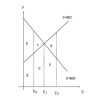
In traditional general equilibrium analysis, Q₁ represents what we would consider equilibrium at P1 (unlabelled). However, using PE, we’re going to take a look at TNSB at each level of Q.

Let’s take a look at Q₀. The area under the Demand Curve (MSB) is A+B. This represents the TSB for gasoline. The area under the supply curve (MSC) is B. Subtracting TSC from TSB leaves us with a TNSB of A. Following the methodology for Q1, we get a TNSB of A+C, which is obviously more optimal than that of Q₀. In this case, the highest TNSB occurs at the market equilibrium Q₁.

Another Look at Market Efficiency

For comparative purposes, let’s take a look at another example and examine the various surpluses that arise and what that means for equilibrium:

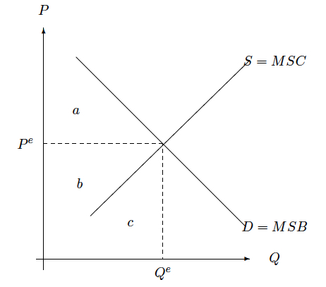
It is also relatively easy to see how we can look at the surpluses generated at the different levels of Q and assign these surpluses to either producers or consumers. Looking at the above market equilibrium chart, we can see that the consumer’s surplus in this case is the value of purchases to consumers (total benefits) minus the cost paid. Consumers received value of ABC, and paid BC, leaving the consumer surplus of A. The producer surplus equals total payments received (B+C) minus the opportunity cost of the production of the goods (C), leaving the producer surplus at B. The TNSB of this situation is the sum of the producer and consumer surpluses (A+B). It is important to note that:

• Market equilibrium requires MSB=MSC,

• Supply equals Demand, and

• Assuming no externalities, market equilibrium represents a Pareto optimum (as illustrated above).

In the next installment we’ll apply the concept of PE analysis to the notion of an additional tax on each gallon of gasoline sold and determine if in fact this would represent market efficiency.

References: Primer on PE: R. Wigle, Microeconomics: J. Perloff.

Graham Mehl is a pseudonym. He is not an ‘insider’. He is required to use a pseudonym by the policies of his firm when releasing written work for public consumption. Although not an insider, he is astonishingly bright, having received an MBA with highest honors from the Wharton Business School at the University of Pennsylvania. He has also worked as an analyst for hedge funds and one G7 level central bank.

Andy Sutton is a research and freelance Economist. He received international honors for his work in economics at the graduate level and currently teaches high school business. Among his current research work is identifying the line in the sand where economies crumble due to extraneous debt through the use of economic modelling. His focus is also educating young people about the science of Economics using an evidence-based approach.